Is Mathematics Real?

“Physics is mathematical not because we know so much about the physical world, but because we know so little; it is only its mathematical properties that we can discover.” – Bertrand Russell

[Note to readers: Owing to limitations in our hosting platform I’m unable to properly present Greek alphabetical characters, or subscripts, within the body of the text. You’ll see “omega” and “theta” where the corresponding Greek character would otherwise appear, and s0, s1, w0, and w1 which should appear with ‘0’ and ‘1’ as subscripts. Thanks for your understanding.]

Introduction

Some believe mathematics is universal, and that mathematical objects exist independently of the mind.  This view contends that we didn’t invent mathematics but instead discovered it.  Others believe mathematics is only as real as any other mental object.  In this blog post I’ll show that the reality of mathematics lies somewhere in between.  I contend that what mathematics describes is universal, and that mathematics relies on what it describes for its own existence.  In this way mathematics, like other objects of mind, is dependently originated.

To make the case we’ll consider a sonar sensor I invented, the genesis of which is purely mathematical.  It was based on a type of radar system called monopulse.  Monopulse radars determine the direction to a radar source, or an object that reflected a radar transmission, from a single (e.g., mono) radar pulse.  A researcher at the University of Texas at Austin extended this idea to sonar.  He published a paper that provided the mathematical foundation for a sensor array concept comprised of several discrete sound-sensing elements.  When the signals from these sensors are combined and processed in a particular way one can determine the direction (e.g., bearing) of a sound source in a rather simple way.

A colleague dropped off a copy of this paper after he learned about research I had done on actuators and sensors for the feedback control of flexible structures.  I immediately made the connection between my work and the monopulse sensor’s mathematical foundation.  This led to an R&D project where I and a few talented colleagues wrestled the concept to the ground and built a prototype sensor that hadn’t been built before.  I received three U.S. patents on the idea, which supports my view that this was a new and unique invention.  And it was based first and foremost on mathematics.

We’ll examine the sensor development as evidence for or against mathematics’ reality.  To do so I’ll summarize the underlying mathematical derivation.  The reader need not be intimidated by the equations that follow; there isn’t a quiz at the end.  Rather I ask that you merely note how the various mathematical variables and functions correspond to statements about concepts in the physical world: pressure, time, distance, angles, sensors, dimensions.  These are all things that we can experience.  Mathematics is a concise way of describing quantities and their various relationships.  Noting the correspondence between what we experience and what mathematics describes lies at the heart of my argument.  If you use this as a guide in your reading the ensuing discussion will flow easily.

Finally, some of you may observe that I’ve limited myself to a particular example based in applied mathematics rather than “pure” mathematics.  I do this because applied mathematics lies in my wheelhouse, whereas pure mathematics does not.  My intuition tells me that the conclusions for pure mathematics would be similar, but let’s leave that for a later blog post.

The Model

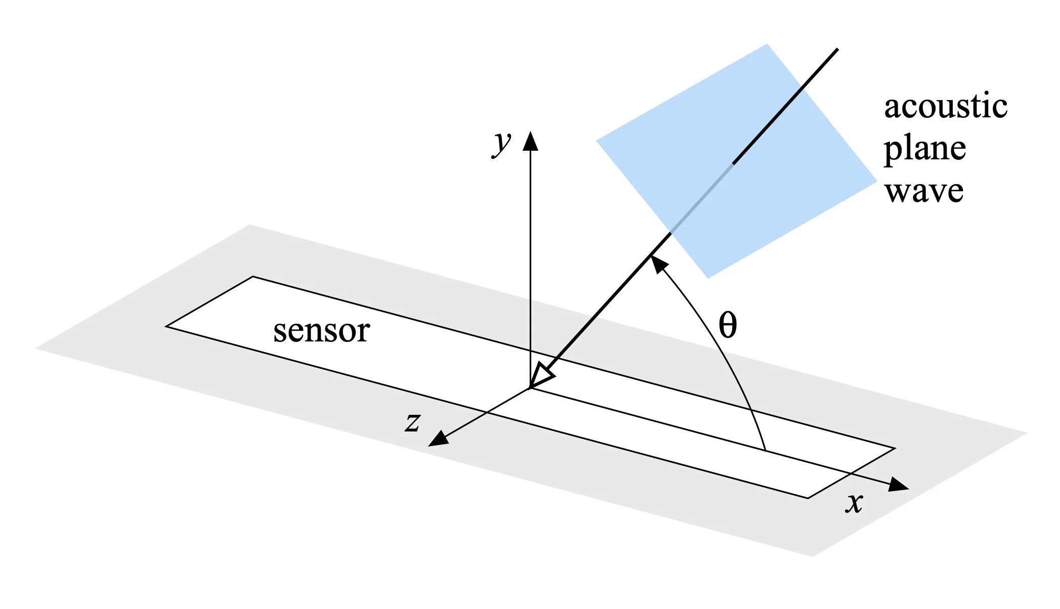
Figure 1: Coordinate system.

Consider the sound pressure wave depicted in Fig. 1.  The wave travels from right-to-left with amplitude P, and can be represented in terms of spatial variables x and y and time t, along with frequency omega, by

where i is the square root of -1.   The wavenumber k is expressed in terms of the sound wave’s angular and circular frequencies omega and f and the sound speed c as

The wavenumber is the spatial analog of frequency; frequency is inversely proportional to the wave’s temporal period while wavenumber is inversely proportional to its wavelength.  The exponential’s argument reflects the wave’s right-to-left movement; for a fixed incidence angle theta and frequency omega, as time t increases distance x must decrease for the argument to maintain a constant value.  Otherwise, the sound wave would spread out (or compress) over time and distance and lose its temporal coherence.

We could have represented the sound pressure wave using sine and cosine functions.  The complex exponential and sinusoids are equivalent, something you can prove using some trigonometry.  More fundamentally, we could even represent the pressure wave as a generic function f of the form f(x + ct).  But the exponential form makes the ensuing analysis simpler, and lends itself to describing more general oscillatory waves via superposition.

The sound wave travels at an angle theta with respect to the x-y axes defined in Fig. 1.  Our goal is to deduce this incidence angle using one or more sensors.  Note that we’ve ignored any z-axis dependence of the sound wave.  We’ll revisit this assumption later, but for the moment consider any variation in the wavefront along that axis as having a spatial scale that is much longer than any other dimension along that axis, such as the sensor’s width.

A rectangular sensor is shown in Fig. 1 that lies in the x-z plane at y = 0.  The sensor’s spatial extent is called its aperture.  Now some of you may ask, “Why is the sensor rectangular?  Don’t you measure sound using microphones, and aren’t microphones circular?”  Many microphones are indeed circular.  But we’ll exploit the rectangular shape and a particular type of sensor in what follows.  For example, piezoelectric ceramics and polymers can have rectangular shapes.  Piezoelectric sensors produce an electric charge over their surface proportional to the applied pressure there – and sound waves are merely time-varying pressures.  

In Fig. 2 we see a sheet of the piezoelectric polymer polyvinylidene fluoride (aka, PVDF). The advantage of this sensing material is that it is flexible and can be applied over large areas, while piezoceramics are generally a couple of centimeters in size or smaller and fragile. The charge is collected over the sensor’s plated area. This plating is connected to electronics that produce signals that we can digitize and analyze.

Figure 2: PVDF sheet with metalized plating.

Returning now to Fig. 1, the sound wave produces a pressure over the sensor’s surface traveling from right-to-left.  If the angle theta is zero, then the sound wave propagates at the speed of sound c along the sensor’s surface.  If theta is ninety degrees – called normal incidence – the plane wave strikes all locations across the sensor simultaneously, which is effectively an infinite speed along the sensor’s surface.  Our piezo sensor produces a charge at every point over its aperture proportional to the local pressure, whatever it may be.  But since the collection electrode covers a wide area, we are not privy to the pressure wave’s spatial details at every point of the aperture.  We can only measure charge summed over the electrode.  Fortunately, we can represent this summing via the mathematical operation of integration, which expresses the sensor output signal s(t) as

The limits of integration ±W and ±L define the sensor dimensions in the z and x directions, respectively; we are summing up the pressure applied over the aperture at each moment in time.  Note that the integration occurs on the plane defined as y = 0.  Consequently, the sin term in the acoustic pressure expression equals zero.  And finally, the constant alpha represents the sensor’s calibration.  It is a factor that represents the sensor material’s sensitivity as well as the gain of any intervening signal conditioning electronics.  Note how the integration “hides” all the sound wave’s spatial information, including its incidence angle.  The output signal s(t) is all we have access to.  We can infer the sound wave’s frequency or frequency content from the signal output.  We can likely infer the sound’s amplitude as well.  However, other details about the sound wave are inaccessible.

Since the integrand – the expression inside the integral – does not depend on z, and factoring the exponential into its spatial and temporal parts lets us rewrite the integral as

the integrand now has a special form.  If the limits of integration ranged from -infinity to +infinity the integral would be a Fourier Transform.  Fourier Transforms are mathematical functions that transform a function expressed in one independent variable into another function expressed in a different independent variable, such as from time to frequency, or space to wavenumber.  The integral above “integrates away” the spatial variable x, and yields an expression in terms of kcostheta, the new independent variable.  (Note that the wavenumber k is a variable, as is the cosine, hence their product is a variable as well called the trace wavenumber.)  But how do we transform an integral with finite limits – here, –L to +L – into one with infinite limits?

We do it by introducing the concept of shading functions, also known as windowing functions.  Referring to Fig. 1 again we note that the sensor aperture is finite, not infinite.  But we can think of this instead as an infinite sensor that only “works” over the finite aperture and has no sensitivity outside it.  This shading or “spatial gain weighting” is constructed using step functions as shown in Fig. 3.

Figure 3: Rectangular shading constructed from two Heaviside step functions.

A step function h(x) is merely a function that “turns on” when its argument goes to zero and equals one afterwards.  Before this transition the function equals zero.  In Fig. 3 the top plot shows a step function that turns on at x = –L, which corresponds to one edge of our sensor aperture.  For values of x less than –L the step function equals zero.  After that it has a “gain” equal to one, all the way to + infinity.  If we want to construct a shading for a finite aperture we need to “turn off” this semi-infinite step function.  The second plot in Fig. 3 depicts a step function that turns on at x = +L, which corresponds to the other edge of our sensor aperture – note how the origin is shifted to the left in this plot.  If we subtract the second step function from the first, we are left with a “boxcar” shading, depicted in Fig. 3’s third plot.  Outside of the range –L ≤ x ≤ +L the shading equals zero.  Inside this range it has a gain of one.  Thus, we can rewrite our integral as

This can be written more generally as

where w(x) is the shading function corresponding to a sensor with finite aperture.  This is a more compact way of representing our rectangular sensor aperture and can be extended to other shapes or spatially varying sensitivity.  More important, we have transformed our expression for the sensor signal output into a Fourier Transform of the shading function w(x).

This is interesting in the abstract, but why do we care? We care because we have studied mathematics and know that Fourier Transforms have some fascinating properties. It’s where we take a creative leap in our analysis, too. You see, if the shading function w(x) happens to equal the derivative of some other shading function w0(x) (we’ll explain derivatives in a moment), our expression for the sensor signal output turns into something wonderful:

Note how the cosine of the sound wave’s incidence angle has popped out of the integral.  This is because of the differentiation theorem of Fourier Transforms: the Fourier Transform of a function’s derivative equals i times the transform variable (here, kcostheta) times the Fourier Transform of the original function. (You can also prove this using integration by parts.) By choosing a particular shading function for our sensor we can gain access to the sound’s spatial (e.g., angle) information.  But how do we separate it from the new shading function w0(x)’s Fourier Transform?

Well, we make another creative leap.  Assume that there is a second sensor, coextensive with the first, that has this shading function w0(x).  Using the analysis above it would have a signal output equal to

If we divide the signal s1(t) by the signal s0(t) we are left with

Eureka!  If we have two coextensive sensors with shadings linked by a derivative, the ratio of their signal outputs is proportional to the direction cosine, and thus the angle of incidence.  The imaginary number i merely represents a phase shift between the sensor signals; engineers can work with that.  Plus the wavenumber k can be written in terms of the sound wave’s frequency and speed, both of which are known (or knowable) quantities.

What would two shadings linked to each other via a derivative look like?  First, recall that a derivative is a calculus operation that computes the slope of a function, e.g., how the function changes with respect to the independent variable.  Consider then the shading w0(x)depicted in Fig. 4.  For values of x less than –L or greater than +L the corresponding sensor sensitivity equals zero.  Since the value of the shading function outside the sensor aperture is a constant (yes, zero is a constant), its slope there is zero.  Consequently, the derivative of the shading w0(x) outside the sensor aperture is zero.  Between –L and 0 the shading has a non-zero and constant slope, hence the derivative of the shading function there is a constant positive number equal to the local slope.  Between 0 and +L the shading has a non-zero and constant negative slope, hence the derivative of the shading function there is a constant negative number equal to the local slope.  Piecing all these bits together results in the shading function w1(x) depicted in the lower half of Fig. 4.  The shading w1(x) is the derivative of the shading w0(x).  The question then is, how do we build a sensor that is actually two coincident sensors that embody these shadings?

Figure 4: Derivative matched shading functions.

Let’s Get Physical

Consider once again the sensor depicted in Fig. 1.  The shading function w1(x) could be realized by simply splitting the sensor into two halves and flipping the sign of signals produced by one half.  That’s perfect doable.  By contrast, the shading function w0(x) corresponds to a sensor with a sensitivity that is zero at one end, rises linearly along its length to a maximum value at its center, then decreases linearly to the opposite end where its sensitivity equals zero.  Note that piezo materials have sensitivities that are nominally uniform over their area, so implementing this shading via a variation in sensor gain isn’t an option.

Recall that we assumed the sound wave was uniform in the z-direction.  This means the sensor experiences a moving sound pressure wave that doesn’t vary across the sensor’s width.  Because of this we can shape a sensor’s aperture as depicted in Fig. 5(a) to approximate our shading w0(x).  The charge collection electrode now has a diamond shape with width that increases linearly from one end, has maximum width in the center, and then linearly decreases to the other end.  This approximates the shading w0(x) depicted in Fig. 4. The derivative-matched shading w1(x) can be constructed using a split aperture like that shown in Fig. 5(b) where one half of the sensor’s output is run through an inverter to flip its polarity.

Figure 5: Shading via electrode shaping.

We could layer these two shaped sensors to build a single device with coextensive, derivative-matched shadings.  Or, more simply, we could take a single piezo sensor and shape its electrodes as shown Fig. 5(c).  We then form the two shadings via suitably summing the outputs of the six sensor elements, as illustrated in Fig. 6.

Figure 6: Sensor shading via element summations.

At this juncture we’ve moved from calculus to a proposed sensor design.  To transition from conceptual design to prototype fabrication is an engineering exercise.  This entails iterative processes for the sensor and associated signal conditioning electronics: design choices, materials and component selection, fabrication, and testing.  For the sensor we found that the electrode pattern shown in Fig. 6 could be constructed using circuit board fabrication technologies.  This obviated the need for custom-plated electrode patterns on the sensing sheet.  We shaped copper electrodes just like you see in Fig. 6 atop a sheet of laminated FR4 glass epoxy, and bonded piezo film to it.  We realized that the opposite side of the sensing element need not have the same electrode pattern.  It only needed a single uniform electrode over its entire surface.  All of these choices were driven by past experience working with similar devices and materials.

The resulting sensor is shown in Fig. 7.  You can see the rectangular sensing element’s outer electrode, covered with a layer of acoustically transparent polyurethane.  This protected the sensor and electrical connections from seawater.  The green material is the FR4 sheet, while the translucent lugs at either end are part of an acrylic housing that contained signal conditioning electronics and a specialized underwater connector.

Figure 7: A real life sensor.

The sensor shown in Fig. 7 was a final prototype; other preliminary prototypes were built and tested along the way to explore the basic functionality.  The next step was to test the device in a controlled environment to validate the concept and explore the sensor’s performance.  We obtained permission to use a large testing pool at a sonar manufacturer based in New Hampshire.  We brought the sensor, mounting fixtures, an omnidirectional underwater sound source, various amplifiers and electronics, and a data acquisition computer.  The basic test setup is depicted in Fig. 8.

Figure 8: Test tank concept.

Testing consisted of placing the sound source and our sensor at opposite sides of the pool, noting the sensor’s angular orientation with respect to the source, then generating a gated 200kHz sine wave that propagated from source to sensor.  Gating means that we took a sinusoidal signal and transmitted it for a short, finite period of time.  This allowed us to determine whether the sensed signal corresponded to the initial sound wave sent from the source or reflections from the pool walls.  Sensor data was recorded for later analysis.  Several data sets were acquired for each angular orientation, then the sensor was rotated by a fixed amount and the process was repeated.  I brought the data back to the office, aggregated the sensor signals as summarized in Fig. 6, and computed the signal ratio to see how (or if) it related to the physical sensor angle settings during testing.  An example of the data is plotted in Fig. 9.

Figure 9: Test data vs. theory.

Fig. 9 is a plot of theory and experiment. The mechanical fixture was rotated a known amount for each set of tests; this defines the plot’s abscissa. In theory the sensor data should describe a straight line on this plot. The estimated angular bearing to the source appears in the ‘+’ data. As you can see the agreement between theory and experiment was remarkably good.

But why did this work?

Discussion

We progressed from calculus, to design concept, to prototype design and fabrication, to test.  A purely mathematical concept was expressed in our sensing device, and it worked as the equations predicted.  While certainly gratifying, it begs the question: Why?  We’ll explore this by first considering the model’s foundations.

First, where does the mathematical expression for sound pressure waves come from?  This is critically important since we’ve based so much of our analysis on it.  The traveling wave expression is a solution of the acoustic wave equation, which we did not present. The wave equation describes how sound propagates in a fluid medium like air or water.  You can think of it as a concise mathematical representation of the rules for sound waves.  If a proposed expression for an acoustic pressure wave does not satisfy these rules, the expression is not a valid representation of sound.  Fortunately, our complex exponential representation satisfies the wave equation – check.  

But where does the acoustic wave equation come from?  The wave equation is derived using mathematics from three branches of physics: fluid mechanics, applied mechanics, and thermodynamics.  From fluid mechanics we use the fact that air is neither created nor destroyed by sound, but the mass of air is conserved, a principle called continuity.  Though expressed precisely using mathematics, continuity is also consistent with our day-to-day observation of the physical world: sound neither creates nor destroys air. 

From applied mechanics we use Newton’s Second Law in deriving the wave equation.  The Second Law links applied force with the rate of change of a mass’s momentum.  It too was formulated using observations of the physical world.  For acoustics the mass is the mass of air vibrating in a sound wave; pressure is related to force by the area over which it acts.  

From thermodynamics we borrow a representation of the state of energy in the sound wave, a mathematical expression that reflects energy conservation.  Conservation of energy is a foundational element of science, developed from observation of the physical world.  

The wave equation is thus a concise mathematical statement of various physical principals, each corresponding to observed phenomena in the physical world.  Or to use a linguistic analogy, the wave equation is a syllogism based upon other syllogisms, each of which is heuristically proven to be true.

Returning to the reader’s guidance offered in the Introduction, note how the various mathematical variables, functions, and equations above all correspond to statements about concepts in the physical world: pressure, time, distance, angles, sensors, dimensions, speed, movement.  Mathematics is a concise way of describing these elements and their relationships.  It’s a language with an exacting grammar.  If a mathematical statement is inconsistent with other correct mathematical statements it is judged to be false.  And within mathematical physics, if a mathematical statement is inconsistent with phenomena in the physical world it is also judged to be false.

So, is applied mathematics real?  When properly practiced, it is as real as our experience of the physical world it describes.  If I drop a rock, the rock falls to the ground.  This commonplace experience can be described by language, and very precisely described using mathematics.  If I make a sound, the sound travels and may be experienced by a listener or measured by a sensor.  In this way mathematics describes what we observe in the physical world – much like language.  

Creating physical devices derived from mathematical principles is merely an extension of the linguistic analogy.  For our sonar sensor there were certainly a few creative leaps.  Ultimately these were associations generated by my mind and the minds of others, all grounded in our experiences of physical reality.  Distributed sensors integrate pressures. Their charge collection electrodes can be shaped to specify spatial sensitivities.  The charge produced on their electrodes can be fed to signal conditioning electronics that produce signals which may be digitized.  A test can be devised to quantify the sensor’s performance.  And software – which itself is a collection of logical statements about quantities – was written to analyze the data.  Each element in this “chain of creativity” was based on logic and real-world experience and thus was consonant with physical reality.  Each can be expressed in mathematical terms.  So, I offer that applied mathematics, properly practiced, is as real as our experience of physical reality. I used it to build a physical device, and that device performed as the mathematics predicted.

But you might ask, “What is mathematics?”  I contend that this metaphysical/ontological question, while interesting, is equivalent to asking, “What is the physical world?” or perhaps more fundamentally, “What is reality?”  I don’t have an answer to any of these questions.  Instead, I’ll offer a favorite quote from the father of modern psychology, William James, which he expressed in the context of religious experience:

“Were one asked to characterize the life of religion in the broadest and most general terms possible, one might say that it consists of the belief that there is an unseen order, and our supreme good lies in harmoniously adjusting ourselves thereto.” [emphasis added]

Interestingly, this perspective is echoed much later by Albert Einstein:

“Try and penetrate with our limited means the secrets of nature and you will find that, behind all the discernible concatenations, there remains something subtle, intangible, and inexplicable. Veneration for this force beyond anything that we can comprehend is my religion.”

I’m not arguing that mathematics is a religion; far from it.  However, our experience of the physical world, carefully considered, reveals an “unseen order.”  I let go of a rock and it falls to the ground and doesn’t fly away in a random direction or remain suspended in air.  Sound propagates from source to receiver.  And so on.  Applied mathematics merely describes this unseen order.  But it does not reveal its genesis – or require any knowledge of that genesis, either.  It is a creation of the mind that describes elements of our experience in a very precise way.  Mathematics, then, has no inherent existence apart from what it describes.  Yet it is as real as the experience of reality that it describes.  For me, that’s enough.

(c) 2021, Shawn Burke, all rights reserved.