Layering Sounds

Our collaboration on Place and Time expands on work I had done the previous Winter in Prague.  I shared several photos and audio snippets from that trip; John was drawn to one pairing in particular.  He observed that a photograph from inside St. Vitus cathedral takes on a spaciousness, immediacy, and subtle energy when accompanied by the corresponding field recording.  The photograph appears below, followed by a clickable audio link.  I recommend listening while softly looking at the photo.  See if you agree that the combination engenders an experience greater than what either component offers by itself.

Figure 1: Inside St. Vitus Cathedral.

Place and Time leveraged John’s photograpy and my audio recordings from a day trip to Portland’s waterfront.  It was our opportunity to try replicating and expanding the “sum greater than its parts” experience I had dipped my feet into in Prague.  You can view and listen to our collaboration at the link below if you haven’t done so already.

Each visual and audio element were recorded at the same place, and at the same time.  The audio soundtrack isn’t comprised solely of single-take field recordings; audio is a bit more mutable than photography.  I layered multiple takes from immediately adjacent locations to expand the sound stage.  In what follows I’ll summarize how I layered two recordings around Portland Light to add width, depth, and interest.  This is a straightforward layering example.  Each component was recorded just around the headland corner from the other, perhaps 5 minutes apart.  

We’ll start with the mix before audio effects are added – just the raw audio with a fade in and a fade out.  The waveforms appear in Fig. 2.  This is a screenshot of the digital audio workstation (DAW) software app ‘Reaper’.  Our example comprises two stereo recordings which are shown stacked in the figure.  The software’s user interface (UI) includes channel strips for each waveform.  As you can see the levels for each channel, represented by the vertical position of the virtual slider buttons, are different.  Reaper allows you to add effects to any channel individually, or to the entire mix.  The latter are called master effects (‘fx’).

Figure 2: Reaper mixing deck software user interface for our project.

The raw mix sounds as follows:

The mix suffers from wind “rumble” and too much low end from the surf – the mix is a bit muddy.  To clean this up I added high-pass filters to each of the two field recordings.  These are implemented using software plug-in modules.  A high-pass filter does just what its name suggests.  Only sounds above a specified frequency are allowed to pass unaltered – the so-called passband.  Sounds below the passband are attenuated.  Fig. 3 shows that the filter was set to pass sounds above 400 Hz, with no additional gain, hence the 0 dB level.  The filter’s “skirt,” defined by the passband’s slope below the corner frequency, has a finite angle.  Filters aren’t like shutters; they don’t completely chop off sound below the corner. Sounds below 400 Hz can still be heard.  They are just de-emphasized, with increasing attenuation as frequency decreases.

Figure 3: High-pass Filter plug-in user interface.

We can then solo either track to hear what it sounds like, as indicated in Fig. 4’s UI screenshot.

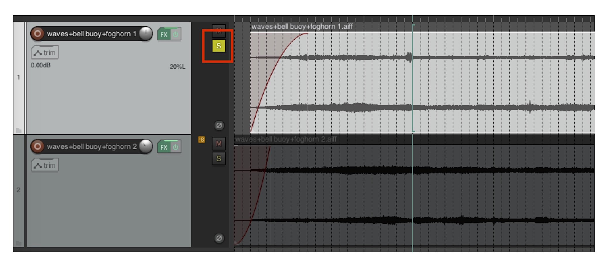
Figure 4: Soloing a track – here, the “left” track.

The first (or “left”) stereo track sounds as follows:

The second (or “right”) stereo track sounds as follows. Note the contrasting elements. There are now sea birds, and the location of the bell buoy and fog horn shift spatially.

Each stereo track is “panned” in the sound stage left or right.  This may sound odd for a stereo track since it’s already in stereo.  Here, panning left means reducing the right channel’s amplitude compared to the left; the left channel’s amplitude is unchanged.  Panning right is just swaps this emphasis.  If the component tracks had been mono, panning would mean moving a single channel to the left or right in the sound stage.  In our example the two stereo tracks are panned symmetrically about center stage.  Their relative amplitude, set by the channel strip virtual faders, was chosen to provide a pleasing blend between the elements.  This part was certainly more art than science.

I noticed that the upper-mid frequency range, spanning ~750 to 3,100 Hz, could stand some tightening up.  The dynamic range in this band, which is the ratio between the softest and loudest sound, was too wide.  This led to less distinct speech elements than I wanted.  So, I added a multi-band compressor to the overall mix.  A compressor is a device – or here, a virtual device plug-in – that takes louder sounds and makes them softer by reducing their amplitude.  The compressor UI shown in Fig. 5 has a nice plot reflecting this variable gain.  The yellow curve shows that as the sound amplitude increases (the plot’s vertical axis), above a specified threshold the compressor reduces the signal amplitude (the fact that the yellow line curves downward).  This compresses the signal’s dynamic range in that frequency band; that’s why they call it a compressor!  Many compressors only work with the overall signal.  A multi-band compressor divides the incoming signal into adjacent frequency bands – here, four – and processes each individually.  The output of each band is then recombined and sent out.  The multiband feature let me target the frequency range I wanted.

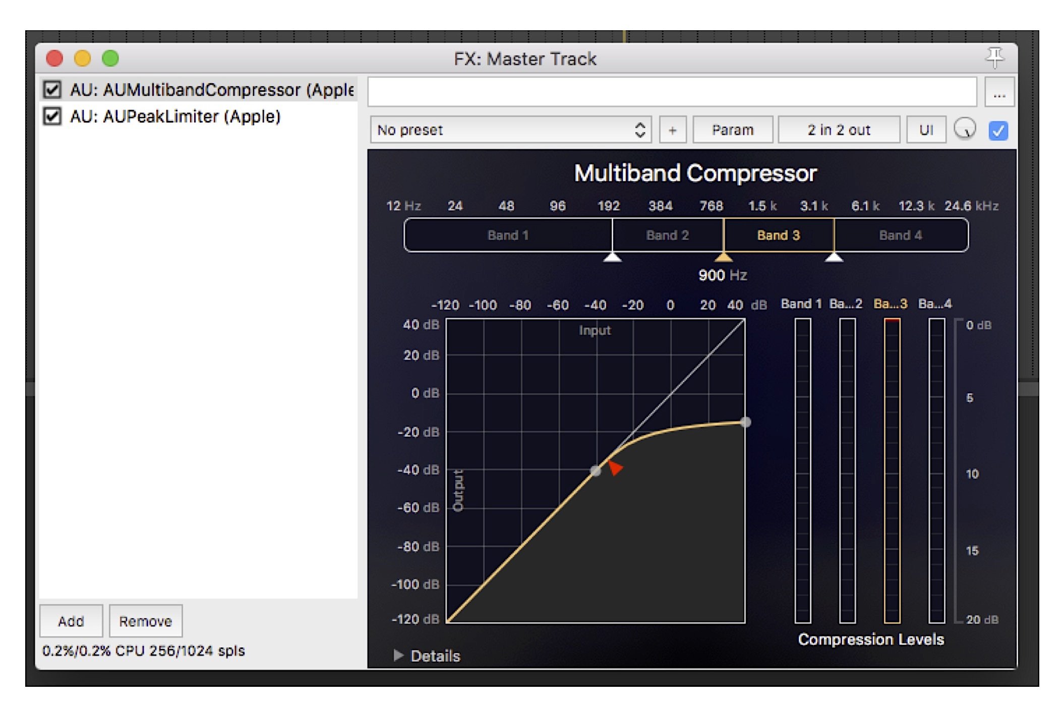
Figure 5: Multiband Compressor master plug-in user interface.

To increase the overall sound amplitude, I could have just turned up the gain.  But this will result in clipping, where the amplitude exceeds the maximum value allowed by the virtual mixing desk software.  Clipping sounds harsh and buzzy; we didn’t want that.  So I added a peak limiter to the overall mix, post-compressor.

A limiter is very similar to a compressor.  But where a compressor lowers higher amplitude signals, a limiter bumps up the amplitude of lower-amplitude signals.  The limiter also implements a nonlinear gain for high amplitude signals just like a compressor.  The peak amplitude is set just below the maximum allowed by the mixer.  This prevents clipping.  The net result is a limiter boosts the signal loudness without clipping.  The peak limiter module’s UI is presented in Fig. 6.  The pre-gain setting was chosen to increase the loudness but not lead to a “squished” sound.  Again, setting this gain is more art than science.  The proof is in the listening.

Figure 6: Limiter master plug-in user interface.

The final mix, including panning, gain setting, high-pass filtering, compression, and limiting sounds as follows:

The sound of the foghorn now appears as two foghorns, one louder (which we interpret as being closer) and one softer (which we interpret as being further away).  The bell buoy and its delightful ringing offer a moody accent.  The surf rises, falls, then builds in intensity.  And the conversation pulls us out from our reverie.  We experience all of this because sound evolves over time.  We add our own narrative.

Text, audio, and images © Shawn Burke, 2022, all rights reserved.